Explaining Seldon decisions with Shapley values

Seldon is Neuralk's tabular foundation model, served through an API. Calling .fit() does not train weights; it uploads the training data as context, and predictions come from in-context learning conditioned on that context. This changes how explainability works. There is no tree ensemble to run TreeSHAP on, no gradients to inspect, and the model runs remotely. This post shows how to compute Shapley-value and Shapley-interaction explanations for Seldon with the Neuralk SDK, on a credit default task, with measured runtimes and credit costs. This post is written for data scientists who are considering using the Seldon API. It assumes familiarity with basic machine learning, but no prior knowledge of Shapley values.

Why explain a tabular foundation model

Tabular models are at the heart of many decision-making processes that can often be treated as consequential by regulation. For instance, the EU AI Act [1] classifies credit scoring of natural persons as high-risk (Annex III); the corresponding obligations, including technical documentation of model logic and transparency to deployers, have applied since August 2, 2026. In the US, ECOA and Regulation B require creditors to state the specific principal reasons for an adverse decision, in what is called an adverse-action notice. The CFPB stated in Circular 2022-03 [2] that model complexity is not a defense. A model that denies a loan application must be able to say why, whatever its architecture.

For gradient-boosted trees this is a solved problem: TreeSHAP [3] computes exact Shapley values in polynomial time from the tree structure. For tabular foundation models the literature is thin. The existing work on TabPFN-style models (Rundel et al. [4]; the TabPFNExplainer in shapiq [5]; the interpretability module of tabpfn-extensions [6]) assumes local access to the model, and often exploits it: features can be removed by editing the in-context training set and re-running inference. Our hosted model exposes directly a wrapper interface around shapiq so that each practitioner can easily access simple explanations of the model behavior without local access to the model.

Shapley values

A Shapley value splits a jointly produced quantity among the parties that produced it. In cooperative game theory the parties are players and the quantity is a payoff. Here the players are the 20 features of one applicant (loan duration, credit amount, checking account status, credit history, etc.), and the quantity is the predicted probability of default for that applicant.

The definition requires a value for every subset of features, not only the full set. Write \(v(S)\) for the model output when only the features in \(S\) are known. Features outside \(S\) are filled from the background dataset, so \(v(S)\) is an average over that dataset rather than a single forward pass. Two subsets fix the scale: \(v(\emptyset)\), the expected prediction when nothing about the applicant is known, and \(v(F)\), the prediction on the complete row.

The Shapley value of feature \(i\) is a weighted average, over all subsets \(S\) that exclude \(i\), of the increment that adding feature (player) \(i\) produces.

\[ \phi_ i = \sum_ {S \subseteq F \setminus \{i\}} \frac{\lvert S \rvert !\,(\lvert F \rvert - \lvert S \rvert - 1)!}{\lvert F \rvert !} \bigl[v(S \cup \{i\}) - v(S)\bigr] \]

The weight has a simple interpretation. Add the features one at a time, in a random order. The weight is the probability that, at the moment \(i\) is added, the features already present are exactly \(S\). So \(\phi_ i\) is the average increase in the prediction caused by adding \(i\), over all possible orders. Summed over all features, the \(\phi_ i\) equal \(v(F) - v(\emptyset)\), the difference between the prediction for this applicant and the baseline prediction. This is the efficiency property. Because of it, each \(\phi_ i\) can be read as the share of that difference due to feature \(i\), in units of probability.

Experimental Setup

We use the German Credit dataset (OpenML data id 31, originally from the UCI repository). Each of the 1,000 rows is a loan application. The task is binary classification: predict whether the applicant is a bad credit risk (300 rows, 30%) or a good one (700 rows, 70%). We call the bad class "default". There are no missing values.

The 20 features describe the loan and the applicant. 7 are numerical and 13 are categorical.

• Loan: duration (months), credit_amount (DM), purpose, installment_commitment (installment as a share of disposable income, on a 1 to 4 scale).
• Financial situation: checking_status, savings_status, credit_history, existing_credits, other_payment_plans, other_parties, property_magnitude, housing.
• Personal: age, personal_status, employment, job, num_dependents, residence_since, own_telephone, foreign_worker.

The median loan is 18 months (range 4 to 72) for 2,320 DM (range 250 to 18,424). The median applicant age is 33. The default rate varies most with the checking account balance and the loan duration:

Savings follow the same pattern as the checking balance: applicants with less than 500 DM in savings default at 33% to 36%, against 13% to 18% for those with 500 DM or more, or with unknown savings. Finally, longer loans tend to be larger: duration and credit_amount have a Pearson correlation of 0.62. This correlation comes back in the interaction terms below.

Computing these values exactly requires the model output for every subset of features. With 20 features there are \(2^{20}\), about one million, subsets, which is too many to evaluate. Instead, the explainer evaluates a random sample of subsets and estimates the values from it. The size of this sample is set by the budget parameter; we use 512 in this post. With \(d\) features, a budget of \(2^d\) covers all subsets and the values are exact (up to the noise from filling in missing features).

The explainer in the SDK

neuralk.explainability.SeldonExplainer wraps shapiq.TabularExplainer [7]. shapiq estimates Shapley values and Shapley interaction indices for any black-box callable. The SDK passes the fitted estimator's predict_proba as that callable. To evaluate a coalition (a subset of "present" features), it imputes the absent features with values drawn from a background dataset, and it batches these evaluations into prediction requests.

The SDK exposes three interaction indices directly: "SV" (plain Shapley values), "k-SII" (k-order Shapley Interaction Index, the default, with max_order=2 for pairwise interactions), and "FSII" (Faithful Shapley Interaction Index [8]). Any other index supported by shapiq is accepted. First-order Shapley values spread joint effects across individual features. Pairwise indices report synergy and redundancy between feature pairs as separate terms. To our knowledge, interaction effects in tabular foundation models have not been studied.

Setup

We ordinal-encode the categorical features because the explainer operates on numeric arrays, and we split 750/250 for train/test.

import os

import numpy as np
from sklearn.datasets import fetch_openml
from sklearn.preprocessing import OrdinalEncoder
from sklearn.model_selection import train_test_split
from neuralk import SeldonClassifier

data = fetch_openml(data_id=31, as_frame=True, parser="auto")
X_raw, y = data.data, (data.target == "bad").astype(int)

cat_cols = X_raw.select_dtypes(include="category").columns
X = X_raw.copy()
X[cat_cols] = OrdinalEncoder().fit_transform(X_raw[cat_cols])
X = X.astype("float32")

X_train, X_test, y_train, y_test = train_test_split(
    X, y, test_size=0.25, stratify=y, random_state=0
)

clf = SeldonClassifier(model="seldon-large", api_key=os.environ["NEURALK_API_KEY"])
clf.fit(X_train, y_train)  # uploads the training data as context

proba = clf.predict_proba(X_test)
accuracy = (proba.argmax(axis=1) == y_test.values).mean()

Test accuracy is 0.764 on this split, with default settings and no tuning. Scoring the 250 test rows is a single prediction request and consumed 1 API credit. The point of this post is the explanation pipeline, not the benchmark.

We build the explainer directly from the fitted estimator:

explainer = clf.explainer(
    background=X_train,
    index="k-SII",
    max_order=2,
    class_index=1,                # explain p(default)
    max_background_samples=None,  # keep the full training set
    feature_names=list(X.columns),
    random_state=0,
)

We pass the full 750-row training set as background and disable the SDK's subsampling option. To evaluate one subset of features, shapiq fills in the missing features with 100 rows drawn from this background (its sample_size default, not exposed by the SDK). This is also why each explanation sends 100 requests. index="k-SII" with max_order=2 asks for one term per feature and one term per pair of features, so that interactions between two features are reported separately (see the Shapley values section). With index="SV", the explainer would return only the 20 per-feature terms. class_index=1 selects the probability of default, the quantity an adverse-action notice has to justify.

Explaining one decision

We explain the test instance the model is most confident about among true defaults: a 48-month loan of 7,119 DM for furniture, from an applicant with a checking balance below 0 DM, savings below 100 DM, no known property, no credit history at this bank, and two existing credits elsewhere. The model assigns \(p(\text{default}) = 0.833\).

# most confident prediction among the true defaults
mask = y_test.values == 1
idx = int(np.argmax(np.where(mask, proba[:, 1], -np.inf)))
x = X_test.iloc[idx]

local = explainer.explain(x.values, budget=512)

explainer.plot_waterfall(local)
explainer.plot_force(local)

The call took 37.5 s, issued 100 prediction requests of 512 rows each, and consumed 100 credits. Building the explainer beforehand issued 2 additional requests (751 rows) to evaluate the empty-coalition baseline over the background; that cost is paid once, not per explanation.

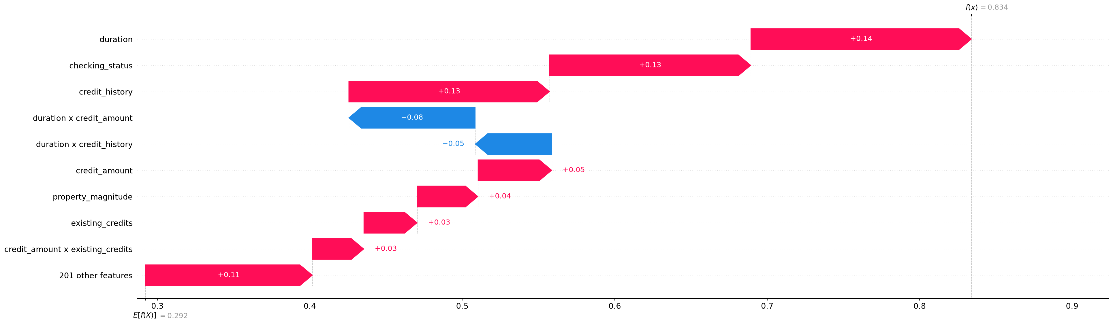
The values can also be read directly from local, without going through a plot: local[(i,)] is the term of feature \(i\), and local[(i, j)] the term of the pair \((i, j)\).

local.baseline_value  # 0.292

first_order = {name: local[(i,)] for i, name in enumerate(explainer.feature_names)}
top = sorted(first_order.items(), key=lambda kv: -abs(kv[1]))[:8]

The eight largest first-order attributions:

The remaining 12 features each contribute less than 0.025 in magnitude. The terms (first-order plus interactions) sum to 0.542, against a 0.541 gap between baseline and prediction; the 0.001 difference is estimation residual at this budget. Read as an adverse-action notice, the top reasons are the loan duration, the overdrawn checking account, and the absence of a repayment record, which is the kind of specific, ranked justification Regulation B asks for.

Interactions

The same local object contains the pairwise k-SII terms, keyed by index pair:

pairs = {k: v for k, v in local.interactions.items() if len(k) == 2}

for (i, j), value in sorted(pairs.items(), key=lambda kv: -abs(kv[1]))[:6]:
    print(explainer.feature_names[i], explainer.feature_names[j], round(value, 3))

The six largest by magnitude:

A negative pairwise term means the joint contribution of two features is smaller than the sum of their individual contributions; a positive term means it is larger. The strongest term, duration with credit_amount, is negative: long loans tend to be large loans, so the two features carry overlapping information and the pair is partly redundant. The pair credit_amount with existing_credits is positive: a 7,119 DM loan on top of two existing credits raises the predicted risk by more than the two facts separately. Both readings are interpretations of the estimated values, not verified properties of the model.

explainer.plot_network(local)

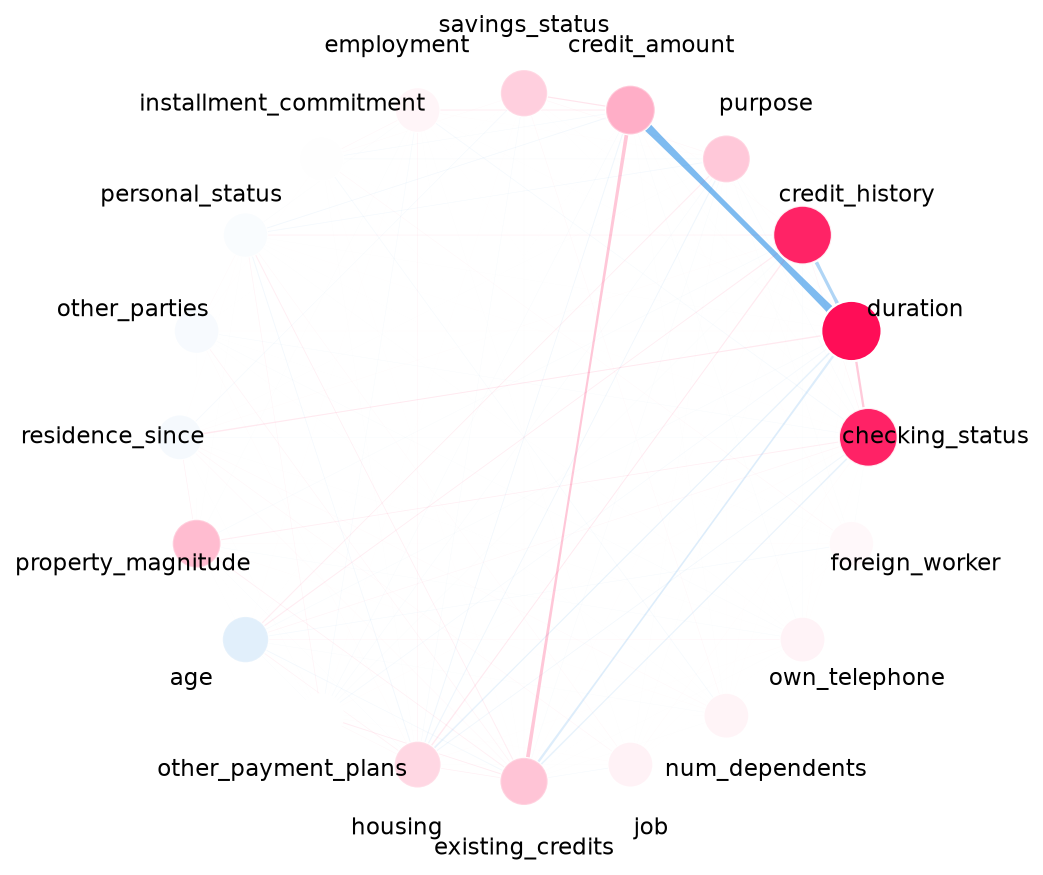
A plain SHAP analysis (index="SV") would fold these terms into the individual attributions, and both the redundancy and the synergy would be invisible.

A global view

explain_global computes one local explanation per row and aggregates them into a global view of which features drive the predicted probability of default across the explained rows. Each row costs one full local explanation, so the input should be a representative subset, not the whole test set.

global_exp = explainer.explain_global(X_test.values[:20], budget=512)
global_exp.feature_importances(normalize=True)
global_exp.plot_bar()

Twenty instances took 1,126 s and consumed 2,000 credits. The ten largest normalized importances (mean absolute first-order value per feature):

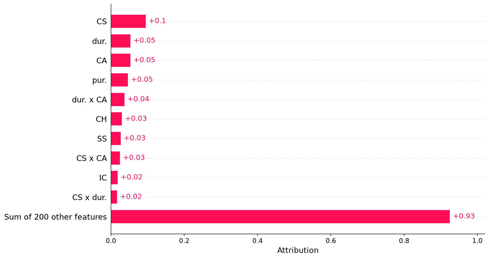
Checking account status dominates, which matches what is known about this dataset. Twenty instances is a small sample; the ranking of the mid-tier features is likely not stable at this size.

Runtime and credit cost

Every number above maps to remote model evaluations, and the API bills one credit per prediction request, so the accounting is direct. In this run:

Each explanation sends 100 requests to the API, one per draw of the imputer, and each request contains budget rows. This is the same for a single explanation and for each row in explain_global. Building the explainer adds 2 requests, once. We observed the same counts with a local model. Increasing budget makes each request larger and the estimate more accurate, but does not change the number of requests. The total cost grows linearly with the number of explained rows. In the global pass, 18 of the 20 explanations took between 36 and 41 s.

One local explanation therefore costs about 100 times a prediction request. That ratio is the price of model-agnostic Shapley estimation against an API, and it is the number to plan around when explanations are needed per decision rather than per audit.

Conclusion

Seldon is only accessible through its predictions, and Shapley values only need predictions, so they can be computed for it directly with the neuralk SDK. On German Credit, the explanation of a single decision gives a ranked list of the features behind it, here the loan duration, the checking account balance and the credit history. The pairwise terms add information that per-feature values do not show, such as the overlap between loan duration and credit amount. Over a sample of applicants, the checking account balance is the most important feature, which is consistent with the default rates in the data.

Practical notes

To explain a decision from a fitted Seldon estimator, build the explainer with clf.explainer(background=X_train) and call explain on the row. For an audit over many rows, call explain_global on a representative sample.

• Index. Use index="SV" if you only need one attribution per feature, for example to list the main reasons for a decision. Use "k-SII" to also see which pairs of features overlap or reinforce each other.
• Background data. Attributions are relative to the background data: the baseline is the average prediction over it. Use data that represents the population you score, such as the training set.
• Correlated features. The default imputer can give misleading attributions on strongly correlated features, here duration and credit_amount. imputer="conditional" is available; we did not evaluate it.
• Training data. Seldon's predictions depend on the uploaded training data. If you change it, recompute the explanations.
• Encoding. The explainer works on numeric arrays, so categorical features must be encoded first, and attributions refer to the encoded columns.

The SDK reference documents the other options.

References

[1] EU AI Act, Annex III (high-risk classification of credit scoring); obligations applicable since August 2, 2026.

[2] CFPB Circular 2022-03, Adverse action notification requirements in connection with credit decisions based on complex algorithms.

[3] Lundberg, S. M., et al. (2020). From local explanations to global understanding with explainable AI for trees. Nature Machine Intelligence.

[4] Rundel, D., et al. (2024). Interpretable Machine Learning for TabPFN. xAI 24.

[5] shapiq documentation, TabPFNExplainer: https://shapiq.readthedocs.io

[6] Prior Labs, tabpfn-extensions interpretability module: https://github.com/PriorLabs/tabpfn-extensions

[7] Muschalik, M., et al. (2024). shapiq: Shapley Interactions for Machine Learning. NeurIPS Datasets & Benchmarks.

[8] Tsai, C.-P., Yeh, C.-K., Ravikumar, P. (2023). Faith-Shap: The Faithful Shapley Interaction Index. JMLR 24.