What is meta-learning? Why is it different from regular ML? And how did it lead to Tabular Foundation Models?
Summary

Look at the seven paintings below. Six are labelled: three by one painter, three by another. The seventh is not.
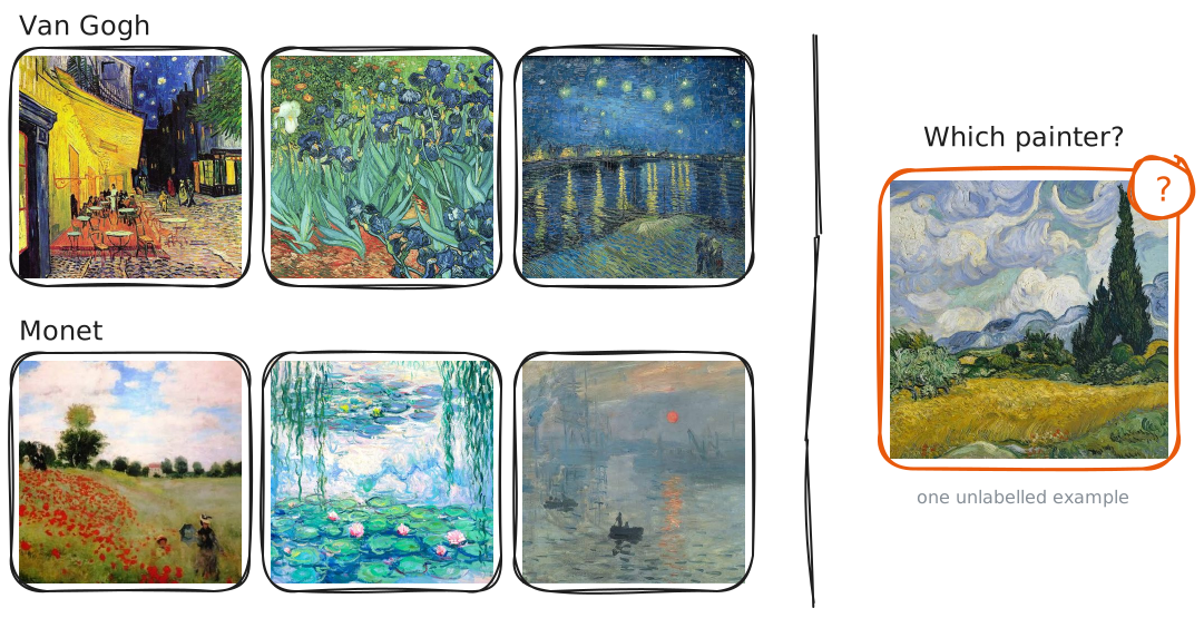
Take a good look, which painter do you think painted the last one? There’s a very high chance that you got the answer right, and in just a few seconds. This is not necessarily because you are an art afficionado and know Van Gogh and Monet’s oeuvre inside out, this is not because you were able to search for more information about both’s techniques, backgrounds and so on. All you had were three pictures of each, you had never been trained on this particular pair of artists and yet somehow, you built an implicit theory of what separates them.
Now imagine having to train a machine learning model to do this same task. It would need a training run: thousands of labeled images of each artist, hours of gradient descent, a validation split, a hyper-parameter search… And at the end you’re left with a model that distinguishes exactly these two painters and nothing else. Hand it a new pair of two it has never seen and the whole process starts again from zero.
This gap is what meta-learning was built to close. When you identified that painting, you weren't drawing on experience with these two painters, you were drawing on a lifetime of telling visual styles apart. You had never solved this task, but you had solved thousands shaped like it. What you brought wasn't the answer, but a procedure for finding answers to questions of this type.
That is the whole idea. Classical machine learning optimises a model to solve a task. Meta-learning optimises a procedure to solve tasks, plural. So a new one costs a glance instead of a training run. We’ll find out later on that this is exactly the paradigm that tabular foundation models are built on.
1. Formalisation of the meta-learning paradigm
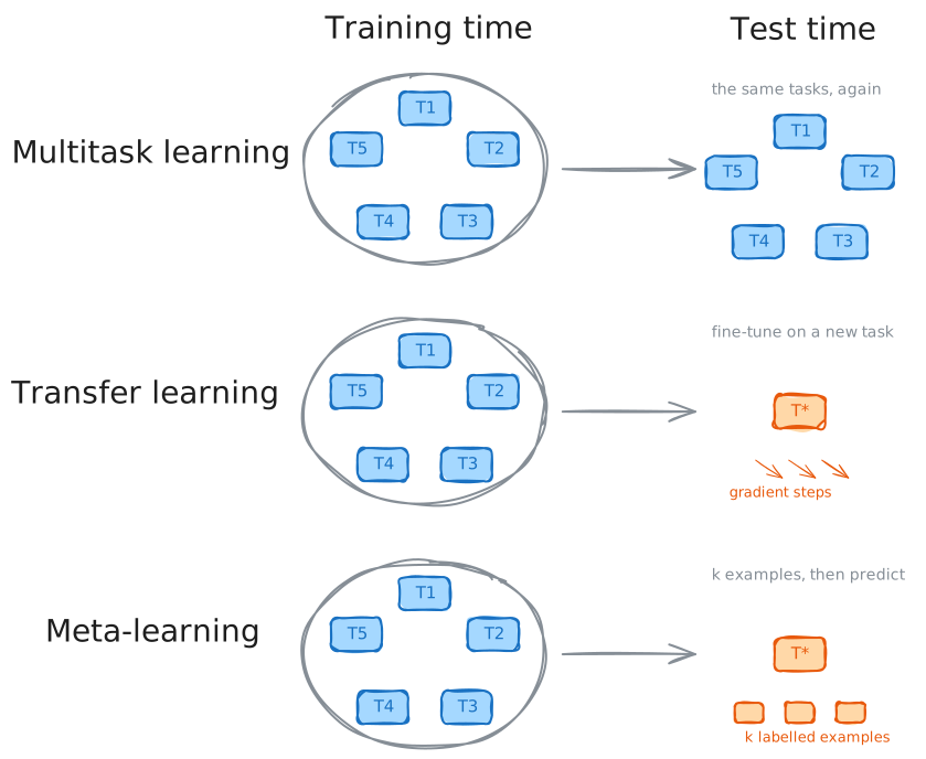
“Learning to learn” is basically meta-learning's catchphrase, but it's a fuzzy definition, and it covers a lot of neighboring ideas. Transfer learning, multi-task learning, and emergent generalization in large models all share the same goal of performing well on new tasks, and the lines between them blur in practice. What sets meta-learning apart is two specific criteria: the training signal comes from a distribution over tasks rather than a single one, and adaptability is explicitly optimized for rather than just hoped for.
These approaches sit close enough to meta-learning that they're often grouped with it, but they don't quite meet both criteria. Here are a few examples:
- Transfer learning/Pretraining then fine-tuning. In this case, a backbone is trained on a source objective (usually on a general self-supervised task) and adapted afterwards by gradient descent. Adaptability is never in the loss. It is a property we hope the representation happens to have, and we find out by trying. This is the closest neighbour and the most common confusion.
- Multitask learning. In this case, one model trained on a fixed, known set of tasks, usually with a shared backbone and one specific head per task. The task set is closed, so a new task means a new head and more training. Adaptation to the unseen is not part of the objective because the unseen is not part of the setup.
Ok now that we have the criteria and understand how they apply, how do we actually implement it? One of the dominant implementations is the double nested loop defined by the MAML (Model-Agnostic Meta-Learning for Fast Adaptation of Deep Networks) framework [1].
Let’s formalize this problem and illustrate it with an example where tasks live in the supervised setting. In order to fit the definition of meta-learning, you need to define the 2 criteria: the task distribution and the inclusion of adaptability in the training objective.
The task and the distribution over tasks: The task is defined by two things: where the data comes from, and how you are graded on it: \(\mathcal{T} = (q(x,y), \mathcal{L})\) where \(q\) is a distribution over labelled examples and \(\mathcal{L}\) is a loss. And each one of these tasks are drawn from a distribution over tasks: \(\mathcal{T}_ i \sim p(\mathcal{T})\).
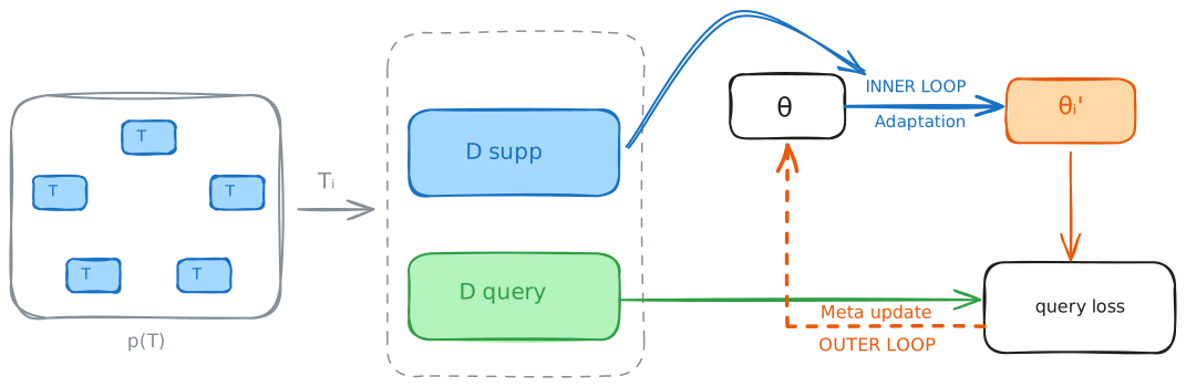
The double loop. MAML formalizes meta-learning as two nested optimization loops. The inner loop adapts the model to a single task, and the outer loop improves the starting point that those adaptations begin from.
Each task is split into a support set and a query set, so we can measure generalization within a task (not yet across the task distribution). Concretely, we sample a task \(\mathcal{T}_ i \sim p(\mathcal{T})\), then draw \(K\) labeled examples from it to form the support set \(D^{\text{supp}}_ i\), and a separate set of examples to form the query set \(D^{\text{query}}_ i\).
• Inner loop: a gradient update on the support set. We represent the model as a parametrized function \(f_ \theta\). An adaptation procedure \(\mathcal{A}\) turns the shared parameters into task-specific ones: \(\theta_ i' = \mathcal{A}(\theta, D^{\text{supp}}_ i)\). In MAML [1], \(\mathcal{A}\) is one (or a few) steps of gradient descent on the support loss, which assumes the loss is smooth enough for gradient-based optimization: \(\theta_ i' = \theta - \alpha \nabla_ \theta \mathcal{L}^{\text{supp}}_ {\mathcal{T}_ i}(f_ \theta)\)
• Outer loop: a gradient update on the query set, through the inner update. We then evaluate the adapted model \(f_ {\theta_ i'}\) on the query set. This query loss measures how good \(\theta\) was as a starting point for adapting to that task. Summed over a batch of tasks, it gives the meta-objective:
\[ \min_ {\theta} \sum_ {\mathcal{T}_ i \sim p(\mathcal{T})} \mathcal{L}^{\text{query}}_ {\mathcal{T}_ i}(f_ {\theta_ i'}) = \min_ {\theta} \sum_ {\mathcal{T}_ i \sim p(\mathcal{T})} \mathcal{L}^{\text{query}}_ {\mathcal{T}_ i}\big(f_ {\theta - \alpha \nabla_ {\theta} \mathcal{L}^{\text{supp}}_ {\mathcal{T}_ i}(f_ {\theta})}\big) \]
The right-hand side carries the main point: the query loss is a function of the original \(\theta\), through the inner step. So the meta-update \(\theta \leftarrow \theta - \beta \nabla_ \theta \sum_ i \mathcal{L}^{\text{query}}_ {\mathcal{T}_ i}(f_ {\theta_ i'})\) backpropagates through both loops. This is how the outer loop learns to shape the initialization so that a single gradient step from it lands somewhere good for each task.
In short, the inner loop adapts \(\theta\) to each task using its support set, and the outer loop updates \(\theta\) itself so that these adapted models \(f_ {\theta_ i'}\) perform well on their query sets across a wide variety of tasks.
We can apply this formalism to a concrete image classification model. Take images from a 200 bird species dataset for example [4]. We want to obtain a model that can perform well on any given classification task across this database. We first define what a classification task is and our distribution across these tasks. The split is by species, not by image. This is what distinguishes it from a classical ML model. We take 100 species for the meta training, 50 for validation, 50 held out for meta-testing, with no overlap. Following the N-way k-shot protocol defined by Vinyals et al. [5] we create our tasks sampled \(\mathcal{T}_i \sim p(\mathcal{T})\).
- Draw \(N\) species from the meta training pool and relabel them \([1, \ldots, N]\)
- Draw \(k_{\text{supp}}\) images per species into the support set \(D^{\text{supp}}_i\)
- Draw \(k_{\text{query}}\) images per species in the query set \(D^{\text{query}}_i\)
Then the 2 loops operate: you adapt on the \(k_{\text{supp}}\) images (model parameters \(\theta \to \theta'\)), you compute the loss of the adapted model \(f_{\theta_i'}\) on the \(k_{\text{query}}\) images, and backpropagate that into \(\theta\). You sample a new task and start all over again. As you can see, a whole classification task is a training sample for the meta model.
2. Why it stalled in vision
However, if you’ve followed the recent works on the domain of vision, whether it be classification or other task natures, the meta-learning path has slowly been abandoned, even when the goal is to adapt well to the unknown. Why is that?
Meta-learning in all its forms (including MAML [1], Matching Networks [5], Prototypical Networks [7]) became the default answer to few shot image classification between 2016 and 2018, but it slowly left the benchmarks for a few reasons. Many ablation tests realised the story wasn’t fully sticking. Raghu et al. [9] found out through ablation tests that the reason the MAML framework worked so well wasn’t necesarily that the meta-initialization (the \(\theta\) obtained through meta training which would then allow to adapt to an unknown task in a few gradient steps) was well positioned for fast learning but rather that feature reuse was the dominant factor, meaning \(\theta\) already contained generally useful features and the inner loop adaptation did not change the performance much on each task. This led to an algorithm called ANIL which almost removes the inner loop entirely and matches MAML performance. Tian et al [8] went even further, by training a simple baseline: learning a supervised or self-supervised representation on the meta-training set, followed by training a linear classifier on top of this representation, can be more effective than sophisticated meta-learning algorithms.
So this may seem like a dead end for meta learning… but if you look back at the 2 criteria we had set earlier, you find out that both had either not been filled to begin with, or become redundant. Natural images share a substrate: edges, textures, shapes... that appears in all images. This means that two episodes are not necessarily 2 different tasks. This makes criteria one fail because this means the distribution of tasks on image classification collapsed to what could resemble a single one. And this makes the second criteria redundant because a good enough representation can solve all of them, leaving no space for adaptation to improve performance.
3. Why is it a perfect fit for tabular models?
Whereas both criteria fail for vision, this is not the case for tabular data, making meta learning not only possible but necessary. This is where tabular foundation models come in.
What is a tabular foundation model? A single model, pre-trained once, that predicts on a table it has never seen by taking the labelled rows as context in a single forward pass. Tabular foundation models differ in their architectural specifics, but what they all share from the start is a task and training setup that fits exactly the meta-training algorithm we defined earlier.
The task and the distribution over tasks: Unlike text or images, there is no web-scale corpus of real tables to learn from because there are few public tabular datasets, they are very heterogeneous, used in most public benchmarks, and often restricted by privacy, making training on them complex.
Tabular foundation models are therefore pre-trained on synthetic data produced by what the field calls a prior: a distribution over data generators, designed by hand, intended to be broad enough that real datasets look like plausible draws from it. Training samples a generator from this prior, and since all tasks of one same model share a loss (ex: CE loss across all classification tasks), that generator is the task’s specificity. We thus get \(\mathcal{T} = (q(x,y), \mathcal{L})\) where \(q\) is the sampled generator and \(\mathcal{L}\) is the specific loss (ex: CE loss for classification tasks).
The double loop training. Training then follows the same double-loop structure as before. We first sample a task \(\mathcal{T}_ i\) from the prior, then draw \(K_ {\text{supp}}\) rows from its generator to form the support set \(D^{\text{supp}}_ i\), and \(K_ {\text{query}}\) rows to form the query set \(D^{\text{query}}_ i\).
• Inner loop. The model adapts to the support set in a single forward pass. Rather than updating its parameters through gradient descent as in MAML, the weights \(\theta\) stay fixed, and the adaptation happens in the model's internal activations: the attention layers condition the representation of each query row on the labelled support rows. This is what is called in-context learning. The two views are less different than they seem as it has been shown, at least in simplified settings, that transformers can learn to implement gradient-descent-like updates within their forward pass [10]. In-context learning can then be seen as an inner loop that the model has learned to run itself.
• Outer loop. The model's predictions on the query rows are scored with \(\mathcal{L}_{\mathcal{T}_i}\), and this query loss is backpropagated into \(\theta\). The global objective is to minimize it across a wide variety of tasks sampled from the prior:
\[ \min_ {\theta} \sum_ {\mathcal{T}_ i \sim p(\mathcal{T})} \mathcal{L}_ {\mathcal{T}_ i}\big(f_ \theta(x^{\text{query}} \mid D_ i^{\text{supp}}), y^{\text{query}}\big) \]
4. Where does that leave us?
Seeing tabular foundation models as meta-learners changes where the hard problem lies. Architectures and in-context adaptation should keep improving, but what ultimately bounds a TFM is its prior.
A TFM generalizes well to any task its prior covers. That part works. The difficulty is making the prior cover the tables that actually exist. Vision and language inherited their priors from the world while we have to write ours, and every property the model has at inference traces back to a decision someone made about the space of synthetic tasks.
Which also changes what failure looks like. You don’t run the risk of overfitting a dataset since you can draw infinitely many fresh ones. But you can absolutely overfit \(p(\mathcal{T})\). In that case, you fit the task distribution faithfully and still fail on real tables, because the distribution was the wrong one. No amount of held-out validation on synthetic data catches that. It's a specification problem, not a generalization problem, and it's the one worth working on.
References
[4] Wah, C., Branson, S., Welinder, P., Perona, P., & Belongie, S. (2011). The Caltech-UCSD Birds-200-2011 Dataset. Technical Report CNS-TR-2011-001, California Institute of Technology.