Foundation models on structured data: tables vs time-series

Tabular foundation models (TFM) ^[2] and time series foundation models (TSFM) ^[15] are models that share a lot of attributes and that now overlap sometimes in their development and in their use cases. On one hand, TFMs are sometimes used on temporal tabular tasks even if the model assumes exchangeability in the rows ^[8], on the other hand, TSFM builders are now using TFM architectures to build their new models ^{[20, 21]}.

The aim of this blog is to take a deep dive into both of these research areas and draw a clear view of both paradigms.

In the first section (section 1), we introduce the TFMs and explain how they work and which tasks they aim to solve.

Then in section 2 we define temporal data and the forecasting task. We notably describe some time-series stylized facts that make time-series forecasting a difficult problem.

In the third section (section 3) we describe the different main learning paradigms we encounter in time-series forecasting.

Then (section 4) we justify the use of TFMs on temporal tasks, while acknowledging that TFMs can be sub-optimal for some cases, and delimit the cases where they apply to time-series ^[7].

1. What is a TFM and on which type of data is it used ?

What is a TFM ?

A tabular foundation model (TFM) is a prior fitted network ^[1] pre-trained on a set of real or synthetic tables in order to perform zero-shot inference on real tabular datasets through in-context learning (ICL). The datasets the model can be used on can be any tabular data that requires using features to make a prediction on a target column. State-of-the-art TFMs all have transformer architectures. These models have been heavily studied in the last years, mainly because their performances match or beat classical machine learning methods (tree-based models, MLP) on several public benchmarks (TabArena ^[6], TabBench), TALENT ^[10]). While some research teams use real datasets to sample tasks for the pre-training phase, we will focus on the synthetic pre-training choice, preferred by SOTA models ^{[36], [37]}.

To explain how the pre-training phase works, we define a set \(P\) of distributions, and a prior distribution \(\Pi\) on \(P\), where \(\Pi\) is called the prior. To build a synthetic table, we sample a distribution \(p \sim \Pi\) and then build a table \(D_n = (x_i, y_i)_{i \le n} \sim p\) called the context and a test sample \((x, y) \sim p\). We train the model to recover \(p(y \mid x, D_n)\). This means we train the model to minimize the loss:

\[
\mathcal{L}(\theta) = \mathbb{E}_{p \sim \Pi}\,\mathbb{E}_{D,(x,y) \sim p}\big[-\log q_\theta(y \mid x, D)\big]
\]

Where \(q_{\theta}\) is the model parameterized by \(\theta\).

In this setting, the samples \(x_i, y_i \sim p\) are independent, which means that the row order in the final table \(D_n\) does not matter. This assumption can be abusive in some cases, especially when the data has temporal dependencies. (This is why we are making this blog-post ^^).

In practice, the usual "priors" that practitioners use are built using Structural Causal Models (SCMs) ^[5]. This means that each dataset on which the model is trained is built using an SCM that specifies the causal & functional dependencies between the features and the target.

An SCM can be described as the following sampling method:

SCM Algorithm

1. Sample a directed acyclic graph ^[34] that specifies some causal relationship between the nodes
2. Select which nodes on the graph will be the features \((x_1, \ldots, x_d)\) and which one will be the target \(y\)
3. For each node \(N_i\), sample a random function \(f_i\) (Gaussian Process, Neural Network, Trees). The node's value will be: \(N_i = f_i(\mathrm{PA}_i, \varepsilon_i), \quad \varepsilon_i \sim p_i\), \(\varepsilon_i\) is noise added to the causal relationship, \(\mathrm{PA}_i\) denotes all the parents of \(N_i\).
4. For each root node \(N_{\text{root}}\), sample a random variable \(\epsilon \sim p_{\text{noise}}\) and assign \(\epsilon\) to \(N_{\text{root}}\)
5. Then use the random functions to successively assign values to each node.
6. Repeat 4-5 \(N\) times to have a dataset \(D_N = (x_i, y_i)_{i \le N}\), \(x \in \mathbb{R}^d\)

The main strength of this algorithm is the diversity of tasks it can sample. The DAG enables to represent any dependence structure between the target and the covariates, and the random functions are chosen to be able to universally represent any function.

Use Cases for the TFMs and the limits of TFM benchmarks

A good way to identify the use cases on which TFMs are likely to be used is to look at the public benchmarks used to compare the models. TabArena is the most widely used, 38 classification and 13 regression datasets. Let's have a look into it. The data in TabArena comes from [OpenML](https://www.openml.org/), a public dataset source that contains thousands of tables. The most represented industries in TabArena are: bank, insurance, marketing, healthcare, pharmacy.

A popular use-case for TFMs is churn prediction. The churn rate is a metric generally used to measure the proportion of customers who cancel a service they were paying for over a given period. It is essential for a company in order to calibrate the price of a new service or to monitor the health of existing ones. On TabArena, 6 tables are churn-like tasks, some synthetic (churn, Fitness_Club), others real (kddcup09_appetency, students_dropout). One can notice that these tables are relatively small (\(\le\) 50k rows), which makes them fertile ground for TFMs. Indeed, TFMs are particularly efficient on small tables, as in-context learning enables them to converge quickly as the context grows.

The TabArena benchmark is however criticized for its lack of task diversity and difficulty. In classification tasks for example, there are 29 datasets out of 38 that contain less than 20k rows, which means that the TFM ranking relies heavily on small table performance. Generally speaking, real client data are under-represented in TabArena datasets and researchers now search for more realistic benchmarks.

Recent articles indeed show that TFMs struggle on some particular tasks (^[9], TabReD ^[8], Beyond IID ^[7]) and that this is especially true on very large tables, or dependent data, which notably include time-series. This has led practitioners to expand the array of evaluation benchmarks (TabBench, TabReD, BeyondArena) for tabular foundation models, in order to cover realistic use-cases as much as possible. Another problem with a persistent frozen benchmark is that it is quickly overfitted ^[6]. Model selection can be done w.r.t. performance on one particular benchmark and is not necessarily robust to generalization to other use-cases.

2. What is temporal data?

Temporal data is data indexed by time. It includes audio signals, weather states, stock prices in finance… Prediction on temporal data means to predict how the data will behave in the future based on what happened in the past. This prediction task is called forecasting. This task can be considered easy if the data is stationary, meaning the temporal dependence structure is invariant by time, and if the auto-regressive structure is "simple".

For instance, let's introduce the Auto-regressive (AR) ^[33] model:
\(X_t = c + \phi_1 X_{t-1} + \epsilon_t\) with \(\epsilon_t\) an independent noise.

When forecasting \(X_t\), the model will just have to find the recursive dependence of \(X_t\) on its direct past value, and the intercept. These models are often used to fit real data and serve as a benchmark of performance ^[13]. They can be extended to linear dependencies with more past values AR(k). A classic textbook example of an AR series is the Lake Huron level forecasting task. Introduced by Brockwell & Davis ^[35] in 1991, the aim is to predict the water level of the lake at time \(t\). The series counts 98 points, 1 per year, and is solved by an AR(2) process: \(X_t = c + \phi_1 X_{t-1} + \phi_2 X_{t-2} + \epsilon_t\).

And the general form of these processes, Auto-Regressive Integrated Moving Average (ARIMA) models, is one of the preferred model choices for time-series forecasting ^{[11, 12]}. Train a foundation model on this family of processes and you'll get a powerful predictive model!

However, why do we want our general model to forecast ARIMA processes if these models can be directly used to fit real data? Well, some data can be nicely fit with auto-regressive linear models and some cannot, we want our model to be good on both situations. This requires a model that can infer quickly the linear auto-regressive behavior when it exists and thus fit the ARIMA coefficients.

And indeed, forecasting time-series can be quite hard, for instance when the time-series has a long term memory, when it has non linear past dependencies, when the event we want to predict is rare etc. In finance for example, predicting the returns of a stock is almost impossible. The magnitude of the signal is very low, the number of exogenous covariates can be huge and the distribution of the data can change over time.

Generally speaking, time-series forecasting is a hard task because real temporal data is never stationary in practice, and contains distribution shifts. This implies that the distributional structure that we aim to learn on a train set or a context set may not be the same on future samples. Suppose that we have a univariate time-series \(y_t\), let's say that the context period is \([0, T]\) and the test period is \((T, T+H]\). We want to use a fixed-length window of past values to predict the next value of the time-series. The target distribution is: \(p(y_t \mid y_{t-1}, \ldots, y_{t-k})\)

Then, one can face several challenges when using the first part of the series \(y_{[0,T]}\) to generalize on fresh samples.

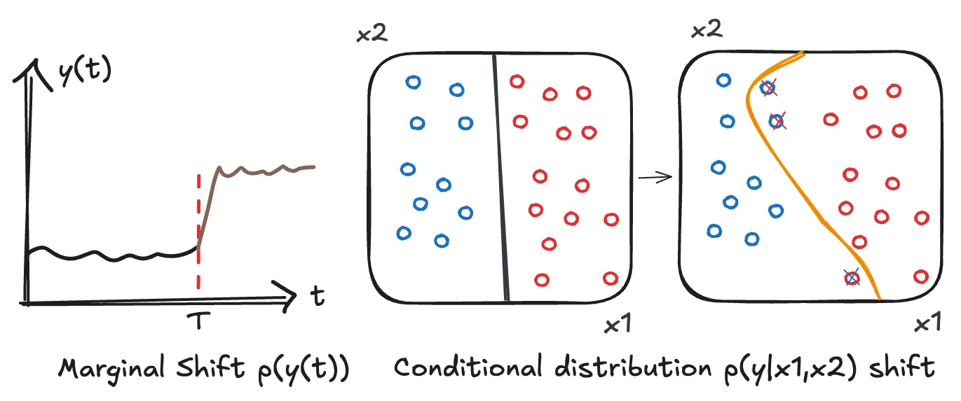
First, marginal distribution shift. The observed marginal distribution of \(y_t\) can change between those two periods (Fig 2), and there are two reasons that can lead to this observation.

→ The true distribution of \(y_t\) can effectively change over time, for example one can imagine an AR(1) model with \(\phi_1 = 0.2\) for \(t \le T\) and then that the series shift to a more autocorrelated behavior with \(\phi_1 = 0.9\) for \(t > T\). The only robust technique to address this problem is to have enough knowledge on \(y_t\) to select a time-period during which \(y_t\) is approximately stationary.

→ \(y_t\) is stationary, but has explored different parts of its space during train and test period. Since the process \(y_t\) shows autocorrelation with past values, the time under which \(y_t\) will explore enough of its whole space in order to have a clear idea of its marginal distribution is much larger than for i.i.d. random variables.

Second, conditional distribution shift. For this case, let's introduce a covariate series \(x_t\) that can be either exogenous or a mix of lagged statistics of \(y_t\) and exogenous covariates.

The target distribution is: \(p(y_t \mid x_{t-1}, y_{t-1}, \ldots, y_{t-k})\). The "features" of the problem are: \((x_{t-1}, y_{t-1}, \ldots, y_{t-k})\) for \(t \in \mathbb{R}\).

The conditional regression function \(y_t = f(x_{t-1}, y_{t-1}, \ldots, y_{t-k})\) can be time-dependent. Which means that the relation we are trying to learn between \(y_t\) and its features can change over time. In finance for example, during down market shocks, stock returns tend to be more correlated to market movements ^[14] than in general. Distribution shifts are hard to model and forecast ^[28], and often require modelling complex and long-range dependencies to make them predictable, which is why learning the full joint distribution of the series is necessary.

‍

3. Foundation models in time-series, the different learning paradigms

Time-series foundation models can target different learning objectives. The first models (Chronos ^[15], Toto ^[17]) were directly inspired by LLMs. Indeed, predicting a fresh sequence of word-tokens by looking at an ordered sequence of previous ones seems very similar to predicting the future trajectory of time-series by looking at the first timestamps ^[22]. This is why auto-regressive models were very popular at the beginning of TSFM development ^[19]. Later, practitioners raised the need for the model to be able to use covariate series that could carry some signal not located in the series itself. The new models (Chronos-2 ^[16], Toto 2.0 ^[18], TabPFN-TS ^[20], ApolloPFN ^[21]) now include covariates in their paradigm.

Autoregressive models. (Chronos-1, Toto) Here, the target distribution is \(p(y_{t,t+h} \mid y_{<t})\), \(y\) can be univariate or multivariate. The model learns to forecast the next token based on past examples, and is therefore learning the joint distribution of the series. This learning-task is very close to LLMs!

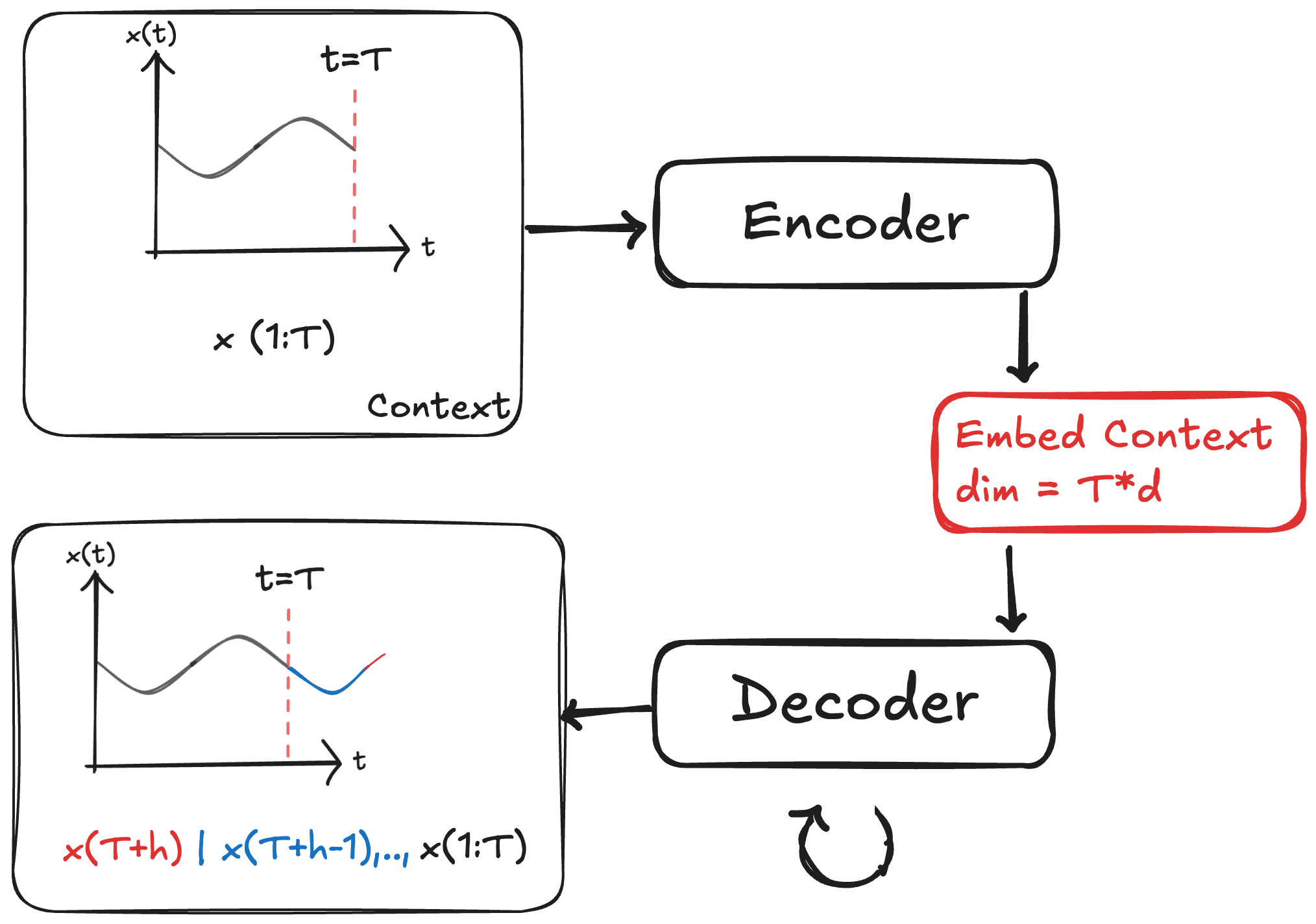
In LLMs the tokens are words, or parts of words. In time-series they are the value of the series at a given timestamp. In LLMs, sequences are sentences and show a structural ordered dependency that is "analogue" to time-series ^[22]. Thus, some of the first time-series foundation models had a classic encoder-decoder LLM architecture ^[15] (fig 3): an encoder that maps a context input to a continuous representation, and then a decoder that successively predicts the next token using the input representation and the previous decoded tokens. These first pure-autoregressive models were a good proof of concept that time series can be forecast by a foundation model. Let's see the architectures that followed.

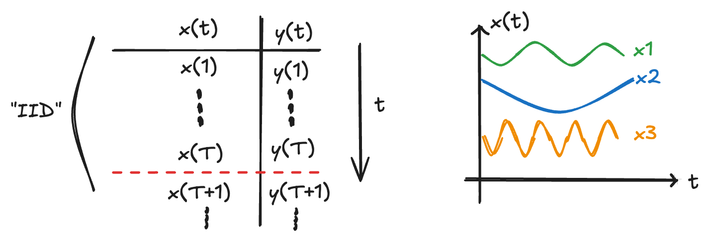
Tabular model extension for time-series. The first prominent example of this framework is TabPFN-TS. This model forecasts univariate time-series well without learning the joint temporal distribution of the series. In this framework, the model is:

\(y_t = f(\tau_t) + \epsilon_t\), with \(\tau_t : t \to \tau(t)\) a function of time, \(y_t \in \mathbb{R}\) (univariate forecasting).

Because a TFM (that we recall ignores row order) doesn't learn the temporal distribution of a series, we must find other strategies. A time-series is first of all a function of time. Trying to find the best "time-representation" to enable the model to find the best relationship between the series and \(t\) seems to be a good idea.

The goal in TabPFN-TS is to have the richest representation of time as features (covariates). This is done by using the context to extract the richest seasonal periods from the target series \(y_t\) (Fourier transforms), adding classical temporal features (month, weeks,...) and some other engineered features that will be useful to build \(\tau_t\) and understand how the data depends on time.

For instance, let \(y_t\) denote the time-series we want to forecast, and assume \(y_t\) follows a hidden periodicity model: \(y_t = a_1 \cos(\omega_1 t) + b_1 \sin(\omega_1 t) + \epsilon_t\). Then, one can compute the periodogram of \(y_t\),

\[
I(\omega) = \frac{1}{n}\left[\Big(\sum_{t=1}^{n} y_t \cos(\omega t)\Big)^2 + \Big(\sum_{t=1}^{n} y_t \sin(\omega t)\Big)^2\right]
\]

find \(\hat{\omega}_1\) by locating its spike, and add as features on the dataset \(x_1(t) = \cos(\hat{\omega}_1 t)\) and \(x_2(t) = \sin(\hat{\omega}_1 t)\). Then one can solve \(y_t = f(x_1(t), x_2(t)) + \epsilon_t\). Here \(f\) is linear which makes it a simple regression problem.

This framework has been built to enable any TFM to make predictions on temporal data. Here, the model assumes that the rows of the context are exchangeable, which means that it doesn't models the temporal structure between rows. Instead, it uses the different deterministic functions of time to exhibit a richer representation \(\tau_t\) of time to help find the correct function \(f\).

TabPFN-TS however under-performs SOTA models on classical time-series benchmarks (GIFT-Eval), where autoregressive models ^{[16, 18]} currently lead.

Hybrid covariate aware paradigm. (Chronos-2, ApolloPFN) Recent models support covariate integration to improve the prediction. However, integrating covariates doesn't necessarily mean that we drop the auto-regressive learning, these models therefore handle both. The target distribution is now:

\(p(y_{t,t+h} \mid x_{t,t+h}, D_{<t})\), where \(D_t = (x_s, y_s)_{s<t}\) is the context, and \((x_t)_t\) is the covariate path.

Both processes \(y_t\) and \(x_t\) can be multivariate. The goal of this paradigm is to infer, using the context, the joint conditional law of the target path, i.e., the temporal dynamics of \(y\) (its dependence on its own past) and its functional response to the covariates (the regression link \(x \mapsto y\)). In this setting, the covariates must be known in advance, which means that \(x_t\) is a known deterministic function of \(t\) on the segment \([T, T+h]\). As in TabPFN-TS, covariates can be deterministic functions of the timestamp like sinusoidal calendar encodings (day-of-week, month-of-year), or exogenous variables whose future trajectory is known at \(T\).

One common example is planned prices, as a retailer sets product prices weeks in advance. The M5 dataset (Walmart, 2020) illustrates this framework: the goal is to forecast the daily unit sales of about 3,000 products across 10 stores over a 28-day horizon, and the selling price of each product is provided for the whole horizon, since it is set ahead of time by the retailer.

When the covariate \(x_t\) is stochastic, for example \(x_t\) is a statistic of \(y_{t-k}\) or an exogenous series whose future is unknown, the Chronos-2 model offers the possibility to use it as "context covariate" (called past-only covariate in the paper), meaning that the distribution being learned is: \(p(y_{T,T+H} \mid y_{1,T}, x_{1,T})\). We want to infer the future of \(y_t\), by using its own past and its past multivariate relation with \(x_t\). For example, consider that you want to predict electricity consumption in Paris. A natural covariate for this task is the outdoor temperature. Because of the thermal inertia of buildings, a cold day keeps driving heating demand into the following one, so the past of the temperature carries information about the future of electricity consumption.

Use-cases in time-series. As for tabular data, let's look at the most used benchmark to draw a landscape of the type of data that can be forecasted by TSFMs. The most widely used benchmark, GIFT-Eval ^[23], contains 23 datasets spanning seven domains: energy, economy/finance, healthcare, transport, nature, sales, and web/cloud operations. The best zero-shot models (non agentic) are TimesFM-3, Toto 2.0 then Chronos-2 for now. GIFT-Eval is criticized mainly for contamination issues: the benchmark authors themselves acknowledge that Chronos and TimesFM were pre-trained on data partly present in GIFT-Eval. Another limiting feature is that no GIFT-Eval dataset provides covariates; see TIME ^[31], fev-bench ^[32] and BOOM ^[17] for more diverse tasks.

4. How and why non-temporal TFMs are applied to temporal datasets ?

Even if TFMs seem sub-optimal for forecasting because they don't learn the temporal distribution of the target \(y_t\), they are directly used for prediction tasks on temporal data. TabRed for example is a tabular benchmark in which several datasets present temporal structure. In fact, TFMs can be a reasonable model for some temporal data.

Suppose that the data we want to forecast is a k-order Markov Chain, meaning that:
\(p(y_{t+1} \mid y_{1:t}) = p(y_{t+1} \mid y_t, \ldots, y_{t-k+1})\).

In this framework, the window \((y_t, \ldots, y_{t-k+1})\) is considered to be a sufficient statistic for \(y_{t+1}\), meaning that all the signal is located in a finite number of past values. We can thus train the model to learn only \(p(y_{t+1} \mid y_t, \ldots, y_{t-k+1})\) instead of \(p(y_{t:t+h} \mid y_t, \ldots, y_1)\).

This case is convenient for TFMs because it can be represented as a tabular task and allows for the model to skip row dependencies. Each row is an example of the distribution \((y_t \mid y_{t-1}, \ldots, y_{t-k})\) and allows the model to learn the conditional dependence between \(y_t\) and its past values. Even when the series is not markovian, it is common to build a fixed-window conditional task to search for the signal.

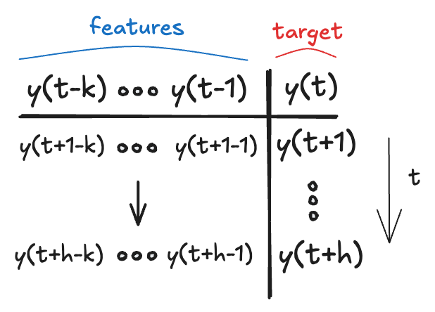
This situation is often extended to more sophisticated models, where we wish to apply transformations to past values of a series \(y_t\) in order to exhibit clearer signal. The model is then \(y_t = f(\phi(y_{t-1}, \ldots, y_{t-k})) + \epsilon_t\) where \(\epsilon_t\) is an independent noise, \(f\) does not depend on \(t\) and \(\phi(y_{t-1}, \ldots, y_{t-k})\), the feature engineering, is in \(\mathbb{R}^d\). If the signal is highly concentrated in a small number of past values, meaning that \(\phi(y_{t-1}, \ldots, y_{t-k})\) is expressive and carries almost all the signal, then the tabular framework can be preferred over the full sequence modelling approach.

Indeed, the simple I.I.D. regression framework (TFM) aims to find the function \(y_t = q_{\theta}(\phi(y_{t-1}, \ldots, y_{t-k}))\) that best approximates \(f\). This problem is much simpler than finding the full joint distribution. \(f : \mathbb{R}^d \to \mathbb{R}\) is a function that operates in a relatively low dimensional space, whereas learning \(p(y_{t+1:t+h} \mid y_{1:t})\) means estimating a density over \(\mathbb{R}^h\) conditioned on a history whose dimension grows with \(t\), which is a far higher-dimensional problem.

So, solving a time-series problem with a TFM is actually possible, if we pre-build good features!

So.. what is the performance of TFMs on time-series ?

Well, pretty bad actually. In ^[7], the authors show that dependent data, mainly represented by time-series, is a critical use-case where TFMs still struggle against classical ML models like XGBoost.

What's next ?

The field of time-series research is old, and richer than that of tabular tasks. Stochastic processes have been studied for more than a century, and auto-regressive models were introduced in 1927 (Yule, 1927). Yet the first modern zero-shot models were developed in the tabular paradigm, in 2022 ^[1], and time-series foundation models only came after (2023) ^{[19, 24].} Time-series forecasting has benefited a lot from the learnings of LLM development ^{[15, 22]}, since the univariate paradigm shows strong analogies with it. Today, the development of systems in the temporal and tabular settings seems to be converging toward a joint effort. Although the two tasks differ at the probabilistic level, it would not be surprising to see unified models emerge at some point.

One of the reasons why the TFM industry developed later than the broader time-series field is data access. Before the big data era, there was no real reason to think that stochastically modelling tables was a good idea: tables are so diverse and complex, and so specific to each use case. A time series, by contrast, is a better-defined and more generalizable object. Its generating process describes it entirely, and clearly specifies the signal carried by its auto-regressive dependencies. And the univariate forecasting task transfers well from one series to another, since the dimension of the problem is the same. It is not the same case for tables: while copulas can describe the multivariate interactions between columns, they do not natively provide a generating mechanism. And more than that, table sizes systematically vary from one task to the next.

The need for general table-generation algorithms led to SCMs, which now dominate TFM priors. The ability of SCMs to model general dependencies is now well established, and the development of these tools is in turn benefiting time-series priors, see ^{[27], [21], [29]}. In a future blog post, we will cover the different ways of generating processes from SCMs.

Lexicon

• Tabular foundation model: A network pre-trained on many tables, which predicts on a new table without any training.

• Prior: The distribution over datasets from which the pre-training tables are sampled.

• Context: The labelled rows the model is given at inference time, and from which it infers the task.

• Structural Causal Model: A generative model where each variable is a random function of its parents in a DAG, plus noise.

• In-context learning: Adapting to a task by reading examples in the input, with no update of the model's weights.

• Stationary: A series whose statistical properties (mean, variance, autocorrelation) do not change over time.

‍

References

1. Müller, S., Hollmann, N., Pineda Arango, S., Grabocka, J., & Hutter, F. (2022). Transformers Can Do Bayesian Inference. ICLR 2022. arXiv:2112.10510.
2. Hollmann, N., Müller, S., Purucker, L., Krishnakumar, A., Körfer, M., Hoo, S. B., Schirrmeister, R. T., & Hutter, F. (2025). Accurate Predictions on Small Data with a Tabular Foundation Model. Nature, 637(8045), 319–326.
3. Grinsztajn, L., Flöge, K., Key, O., Birkel, F., et al. (2026). TabPFN-3: Technical Report. arXiv:2605.13986.
4. Qu, J., Holzmüller, D., Varoquaux, G., & Le Morvan, M. (2026). TabICLv2: A Better, Faster, Scalable, and Open Tabular Foundation Model. ICML 2026. arXiv:2602.11139.
5. Peters, J., Janzing, D., & Schölkopf, B. (2017). Elements of Causal Inference: Foundations and Learning Algorithms. MIT Press.
6. Erickson, N., Purucker, L., Tschalzev, A., Holzmüller, D., Mutalik Desai, P., Salinas, D., & Hutter, F. (2025). TabArena: A Living Benchmark for Machine Learning on Tabular Data. NeurIPS 2025 D&B. arXiv:2506.16791.
7. Purucker, L., Tschalzev, A., Erickson, N., Blayer, G., Holzmüller, D., Arazi, A., Pfefferle, A., Tajjar, M., Varoquaux, G., & Hutter, F. (2026). Beyond IID: How General Are Tabular Foundation Models, Really? arXiv:2606.30410.
8. Rubachev, I., Kartashev, N., Gorishniy, Y., & Babenko, A. (2025). TabReD: Analyzing Pitfalls and Filling the Gaps in Tabular Deep Learning Benchmarks. ICLR 2025. arXiv:2406.19380.
9. Kim, M. J., Schambach, M., Essenberger, F., Sres, A., & Höhne, J. (2026). Exploring Differences Between Tabular Enterprise Data and Public Benchmarks. arXiv:2606.30452.
10. Ye, H.-J., Liu, S.-Y., Cai, H.-R., Zhou, Q.-L., & Zhan, D.-C. (2024). A Closer Look at Deep Learning on Tabular Data (TALENT). arXiv:2407.00956.
11. Box, G. E. P., Jenkins, G. M., Reinsel, G. C., & Ljung, G. M. (2015). Time Series Analysis: Forecasting and Control (5th ed.). Wiley.
12. Hyndman, R. J., & Khandakar, Y. (2008). Automatic Time Series Forecasting: The forecast Package for R. Journal of Statistical Software, 27(3), 1–22.
13. Makridakis, S., Spiliotis, E., & Assimakopoulos, V. (2020). The M4 Competition: 100,000 Time Series and 61 Forecasting Methods. International Journal of Forecasting, 36(1), 54–74.
14. Ang, A., & Chen, J. (2002). Asymmetric Correlations of Equity Portfolios. Journal of Financial Economics, 63(3), 443–494.
15. Ansari, A. F., Stella, L., Türkmen, C., Zhang, X., Mercado, P., Shen, H., Shchur, O., Rangapuram, S. S., Pineda-Arango, S., Kapoor, S., et al. (2024). Chronos: Learning the Language of Time Series. TMLR. arXiv:2403.07815.
16. Ansari, A. F., Shchur, O., Küken, J., Auer, A., Han, B., Mercado, P., Rangapuram, S. S., Shen, H., Stella, L., Zhang, X., et al. (2025). Chronos-2: From Univariate to Universal Forecasting. arXiv:2510.15821.
17. Cohen, B., Khwaja, E., Doubli, Y., Lemaachi, S., Lettieri, C., Masson, C., et al. (2025). This Time is Different: An Observability Perspective on Time Series Foundation Models (Toto). arXiv:2505.14766.
18. Khwaja, E., Lettieri, C., Woo, G., Belouadah, E., Cenac, M., Jarry, G., et al. (2026). Toto 2.0: Time Series Forecasting Enters the Scaling Era. arXiv:2605.20119.
19. Das, A., Kong, W., Sen, R., & Zhou, Y. (2024). A Decoder-Only Foundation Model for Time-Series Forecasting (TimesFM). ICML 2024. arXiv:2310.10688.
20. Hoo, S. B., Müller, S., Salinas, D., & Hutter, F. (2025). From Tables to Time: How TabPFN-v2 Outperforms Specialized Time Series Forecasting Models. arXiv:2501.02945.
21. Potapczynski, A., Selvam, R. K., Konstantinova, T., Wolff, M., Olivares, K. G., Ma, R., Mahoney, M. W., Wilson, A. G., Oreshkin, B. N., & Efimov, D. (2026). Time-Aware Prior Fitted Networks for Zero-Shot Forecasting with Exogenous Variables (ApolloPFN). arXiv:2603.15802.
22. Gruver, N., Finzi, M., Qiu, S., & Wilson, A. G. (2023). Large Language Models Are Zero-Shot Time Series Forecasters. NeurIPS 2023. arXiv:2310.07820.
23. Aksu, T., Woo, G., Liu, J., Liu, X., Liu, C., Savarese, S., Xiong, C., & Sahoo, D. (2024). GIFT-Eval: A Benchmark for General Time Series Forecasting Model Evaluation. arXiv:2410.10393.
24. Dooley, S., Khurana, G. S., Mohapatra, C., Naidu, S., & White, C. (2023). ForecastPFN: Synthetically-Trained Zero-Shot Forecasting. NeurIPS 2023. arXiv:2311.01933.
25. Kang, Y., Hyndman, R. J., & Li, F. (2020). GRATIS: GeneRAting TIme Series with Diverse and Controllable Characteristics. Statistical Analysis and Data Mining, 13(4), 354–376.
26. Moroshan, V., Siems, J., Zela, A., Carstensen, T., & Hutter, F. (2025). TempoPFN: Synthetic Pre-training of Linear RNNs for Zero-shot Time Series Forecasting. arXiv:2510.25502.
27. Xie, S., Feofanov, V., Alonso, M., Odonnat, A., Zhang, J., Palpanas, T., & Redko, I. (2025). CauKer: Classification Time Series Foundation Models Can Be Pretrained on Synthetic Data Only. arXiv:2508.02879.
28. Helli, K., Schnurr, D., Hollmann, N., Müller, S., & Hutter, F. (2024). Drift-Resilient TabPFN: In-Context Learning Temporal Distribution Shifts on Tabular Data. NeurIPS 2024, 37, 98742–98781.
29. Chen, T., Zhou, Y., Gong, Z., He, H., Li, H., Chen, Z., Wang, D., Zhang, X., Liu, D., Peng, C., Chen, Z., & Ding, W. (2026). Trio: Learning Time-Series Forecasting with Temporal-Spatial-Sample Attention and Structural Causal Priors. arXiv:2606.07291.
30. Oreshkin, B. N., Jauhari, M., Selvam, R. K., Wolff, M., Pan, W., Ramasubramanian, S., Olivares, K. G., Konstantinova, T., Potapczynski, A., Cao, M., Efimov, D., Mahoney, M. W., & Wilson, A. G. (2026). Zero-shot Forecasting by Simulation Alone (SarSim0). ICLR 2026. arXiv:2601.00970.
31. Qiao, Y., et al. (2026). It's TIME: Towards the Next Generation of Time Series Forecasting Benchmarks. arXiv:2602.12147.
32. Shchur, O., Ansari, A. F., Turkmen, C., Stella, L., Erickson, N., Guerron, P., Bohlke-Schneider, M., & Wang, Y. (2025). fev-bench: A Realistic Benchmark for Time Series Forecasting. arXiv:2509.26468.
33. Yule, G. U. (1927). On a Method of Investigating Periodicities in Disturbed Series, with Special Reference to Wolfer's Sunspot Numbers. Philosophical Transactions of the Royal Society A, 226, 267–298.
34. Pearl, J. (2009). Causality: Models, Reasoning, and Inference (2nd ed.). Cambridge University Press.
35. Brockwell, P. J., & Davis, R. A. (1991). Time Series: Theory and Methods (2nd ed.). Springer Series in Statistics. Springer, New York.
36. LimiX Team, Stable AI & Tsinghua University. (2026). LimiX-2: Technical Report. arXiv:2609.17488.
37. Jäger, B.,et al. (2026). TabPFN-3.5: Technical Report. arXiv:2609.17895.

‍